Final pieces of the straight skeleton puzzle

In the last couple of parts, I covered the definition of the straight skeleton, plus some details about how to calculate it with finite precision math. Here I’ll go over some of the final elements of the implementation.

Polygons with holes

We can also calculate a straight skeleton for polygons with holes. In this case, we will start with multiple “wavefronts” – one that represents the outer edges of the polygon moving inwards, and others than represent the edges of the holes, moving outwards. It should look something like the following:

We can advance time on each wavefront independently and they will grow or shrink. Clearly though, at some point they will cross over each other and will we start to get invalid geometry. Somehow the independent wavefronts must interact. Furthermore, if look closely at the diagrams above you may notice that at later points on the timeline, not only do we have fewer wavefronts than we started, but we also have wavefronts that contain some edges from the outer loop and some from the holes. So the wavefront must interact in some way that causes them to merge together – some operation must take 2 wavefronts as an input and produce a single wavefront as an output.

It turns out that the edge collapse calculations are unchanged, but we need to take into account a new “motorcycle crash” case. Motorcycles from one wavefront can now collide with edges from another wavefront. You can see this happening in the diagrams above. In this particular case we only have vertex vs vertex style crashes, but it works the same with vertex vs edge.

Recall that in the earlier single wavefront case, motorcycle crashes always split the wavefront into two. Here, though, we actually have the opposite: we take 2 wavefronts as input and output a single wavefront, containing some edges from the first and some from the second. Otherwise the motorcycle crash calculations are quite similar.

I call this a loop merge event, and it turns out this is the only new interaction we have to support in order to handle polygons with holes. So with this, we’re set to go. The final result should look a little like the following:

Advancing wavefronts together

Supporting this case does have some perform implications: for one, we have to search all loops for motorcycle crashes, not just one. But also it means that we need to advance time on all loops at the same time.

Without this case, wavefronts never interact with each other. That means we can advance time on each independently. This is convenient for implementation because we can focus on one “active” loop at a time. But to find these loop merge events accurately the wavefronts we’re searching through must all be synchronized in time. In other words, we must now advance time for all wavefronts together.

Not only that, but there’s a chance that other events on the loops are happening during the same event window as the loop merge event. In fact, in this example you can see that there are actually multiple loop merge events happening in the same event window! We also need the guarantees here that all events in the window are processed, regardless of what error creeps during during processing the window.

So this means our event window must be a multiple-loop data structure and support edges and vertices changing from one loop to another as a result of processing these events (and actually the simpler single-loop crash event as well). And ultimately, it’s just another example where a seemingly simple feature adds a lot of implementation complexity in this algorithm.

Some performance optimizations

Generally the algorithm for calculating the straight skeleton is pretty quick. The most expensive part by far is finding motorcycle crashes – since this is the only O(M * N) type operation where we have to search through multiple edges for multiple vertices.

Only reflex vertices can cause motorcycle crashes or loop merge events, so that helps reject many cases. But we can also help here by doing a full search during initialization and then just updating events for edges and vertices that have changed. I do this pretty simply – for each new edge created, we compare to all potential motorcycles to see if it happens earlier than the current projection. And if a vertex is projected to crash into an edge when that edge is removed (which should be the result of processing another crash), then we will recalculate that motorcycle from scratch.

Arbitrary polygon inputs

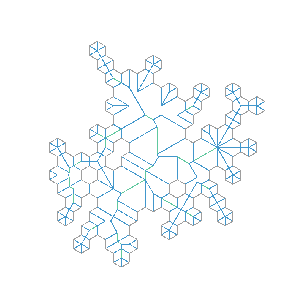
Here are some examples of straight skeletons calculated for arbitrary shapes. The input geometry I’m using here are all sourced from CC0 SVG files (which you can find on freesvg.org).

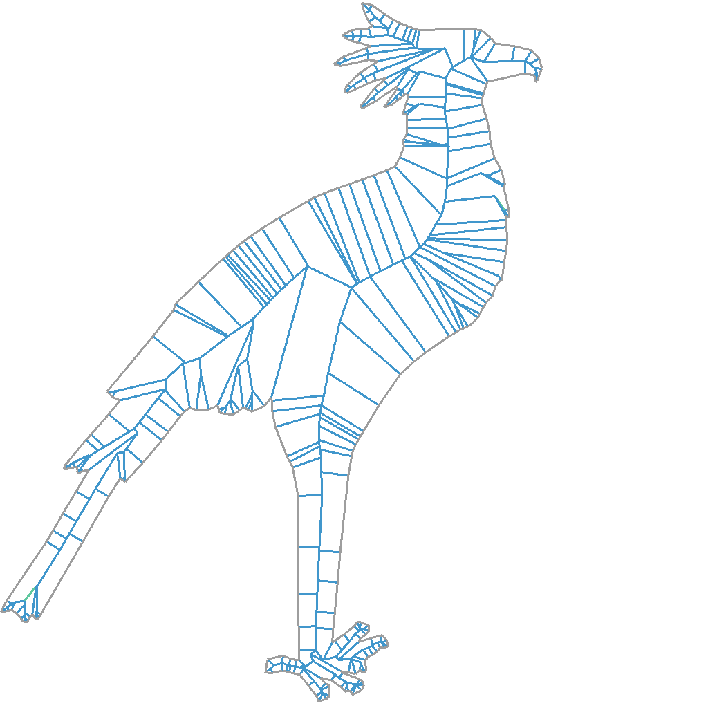
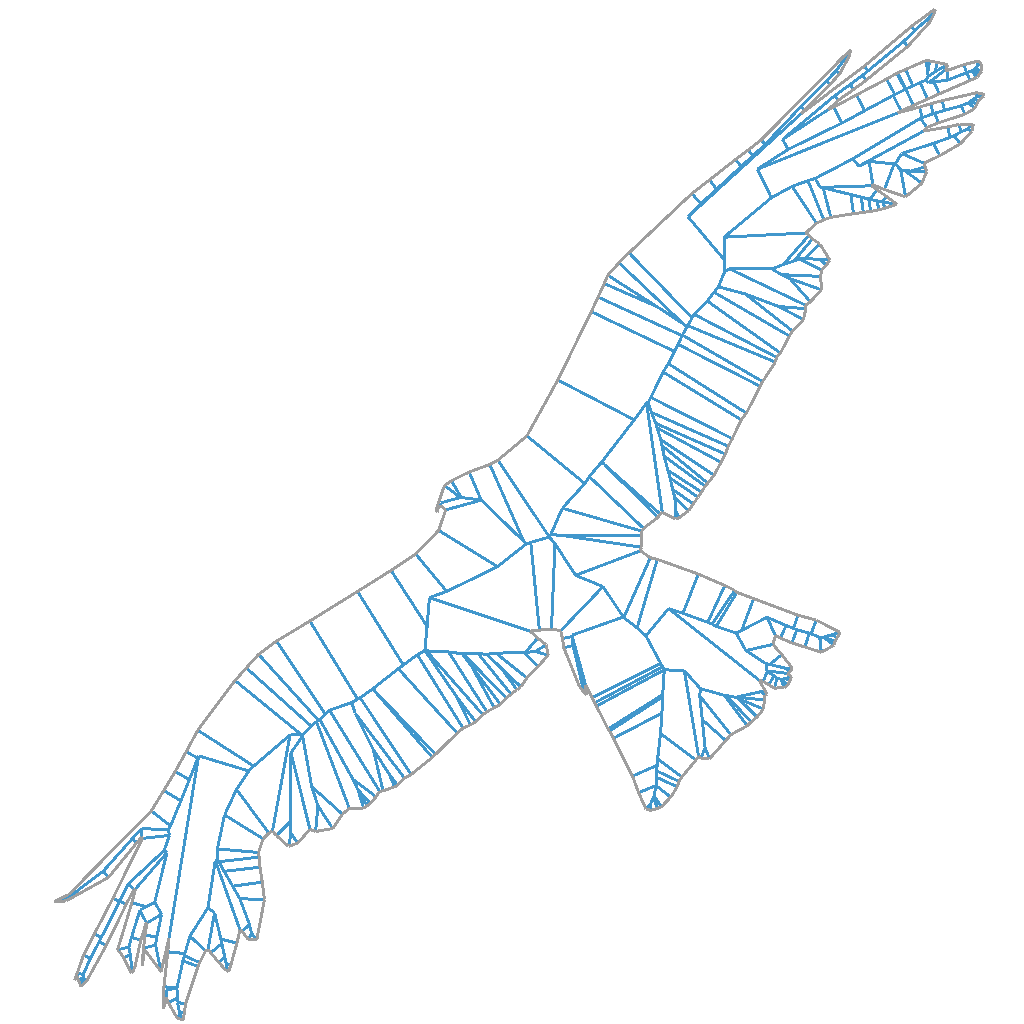
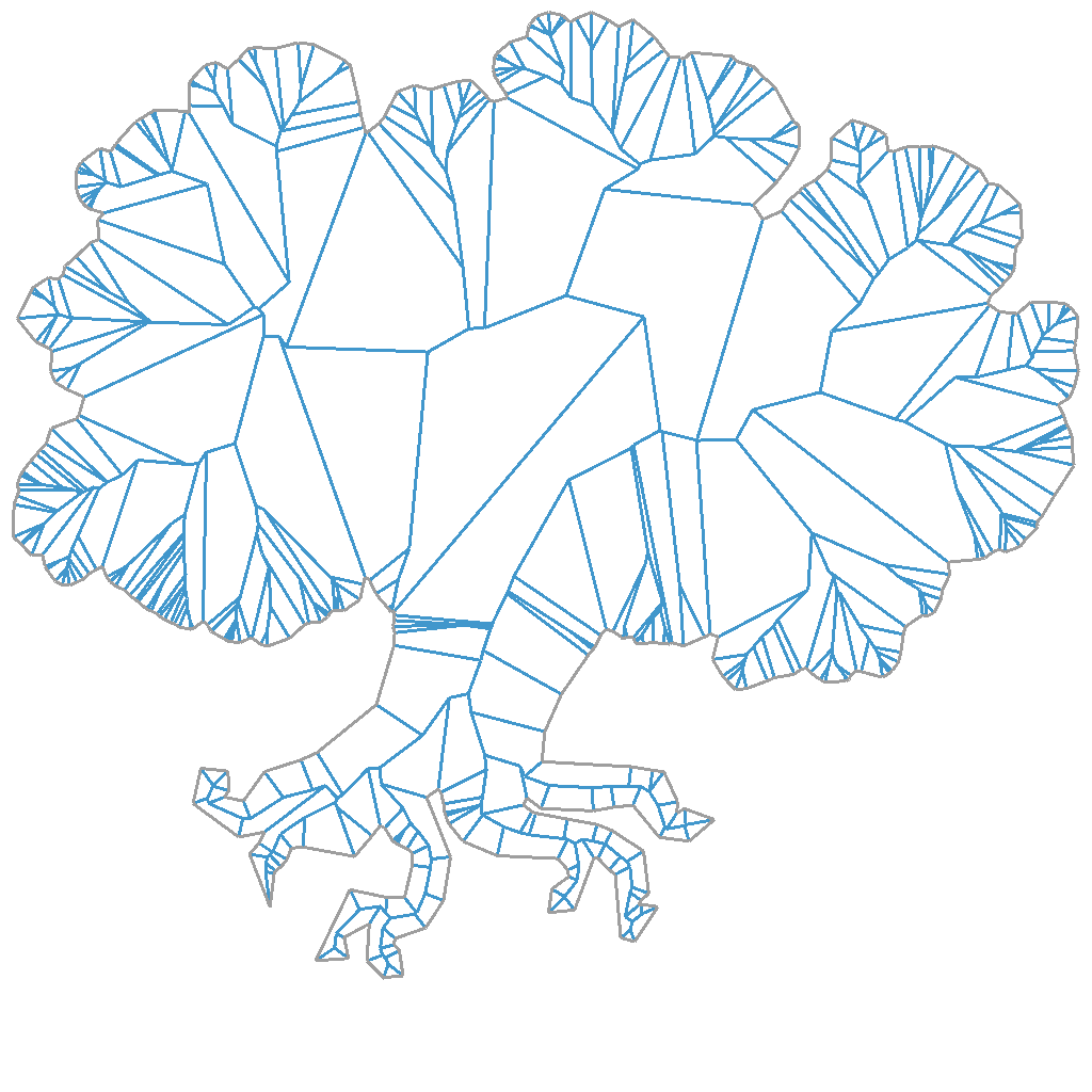
Generally these arbitrary inputs should be easier to calculate than the hex grids I’ve been using. We just need to be careful about near-collinear edges in the input around smooth parts of the silhouette.

One of the interesting properties of the algorithm, which you may notice from the diagrams above, is that smaller non-structural edges tend to result in small polygons traced by the skeleton. But the overall shape of the input is always well represented by the skeleton. It’s not so direct as to say that the structural significance of an edge is proportional to the area of the traced polygon. But what it seems to me is that as time advances in the algorithm, the wavefront becomes gradually simpler in such a way that non-structural details are gradually removed and we’re left with a shape that represents how the input is structurally arranged.

3D outputs

I’ve used the term “time” to talk about the advancing wavefronts. But something really interesting happens if we represent this “time” dimension as a third spatial dimension (recall that we’re using the same units for the time & space dimensions anyway).

More concretely, if we take the time value for when a vertex stops moving and use that for a “Z” value for that vertex, we will end up with a 3D shape.

Before you take a look at the output, here’s something to think about – recall that each edge is moving in the direction of it’s normal at the same rate. Now that we’ve associated time with the Z axis, this will mean that every single edge will have exactly the same slope in 3D, with respect to its tangent. This should mean that the output should look very uniform.

Here’s some quick examples of what that looks like (exported into Blender):

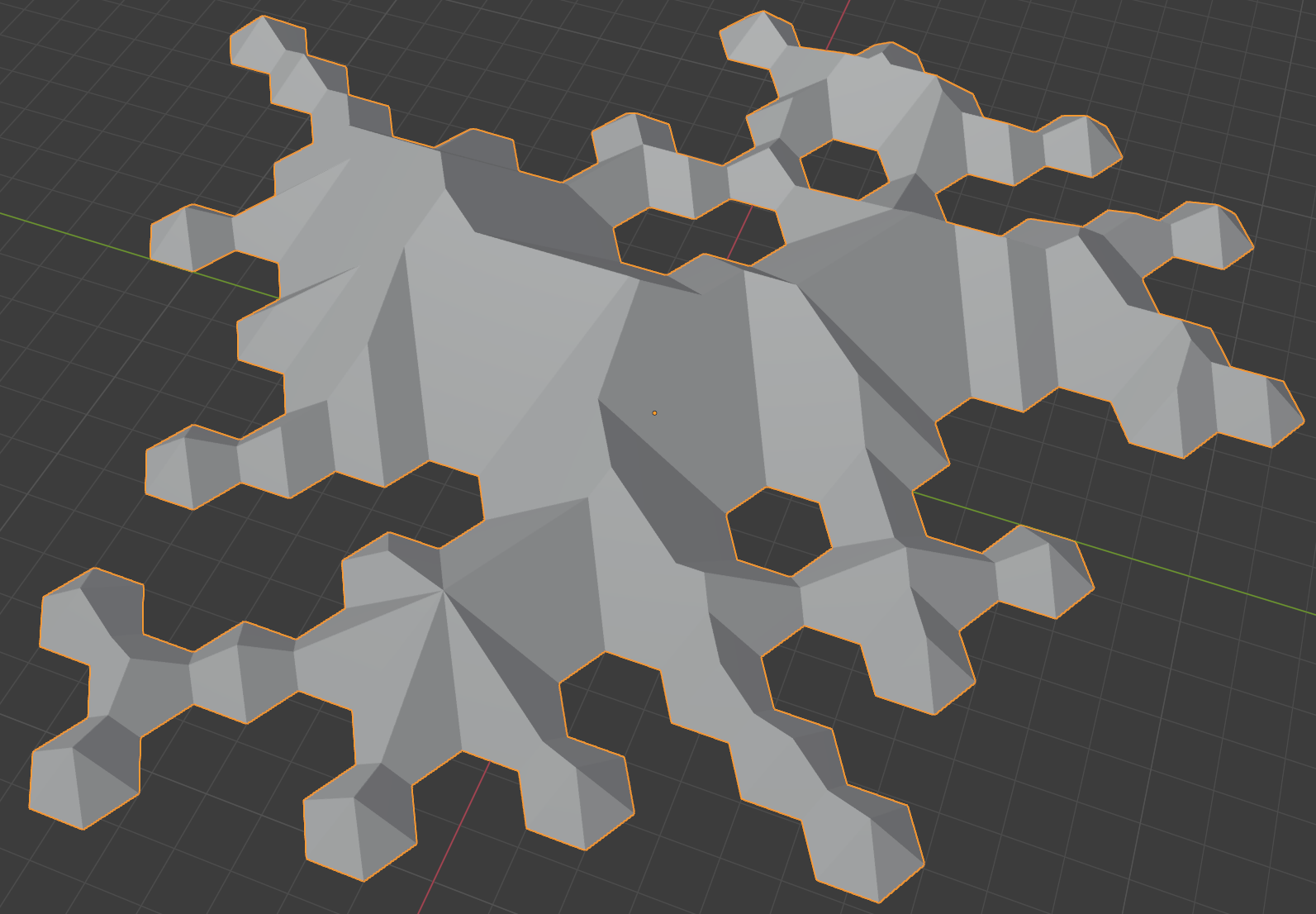
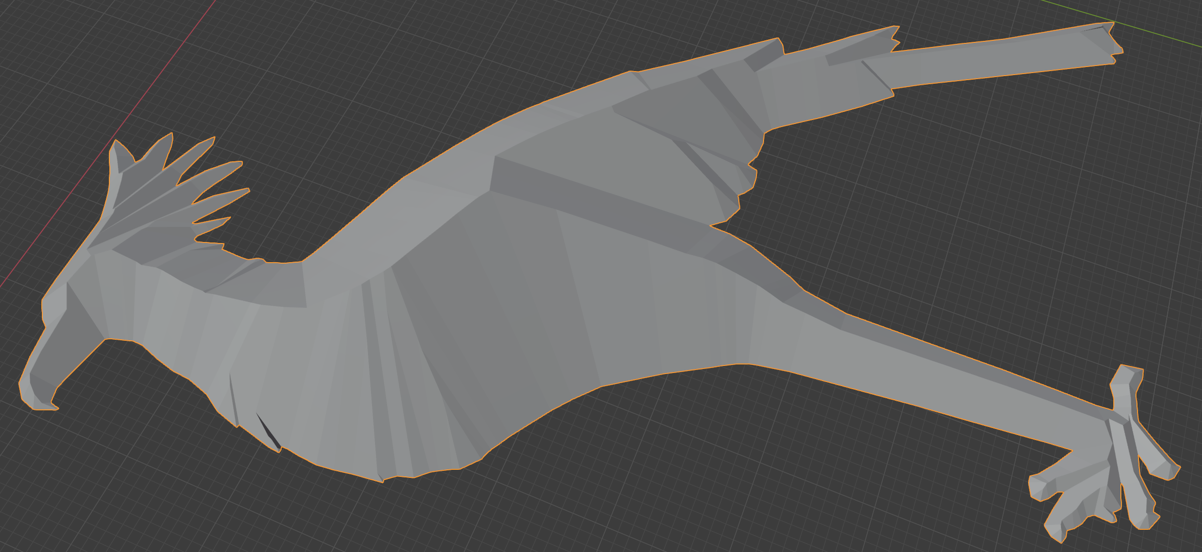
You may notice here the regularity of the slopes in 3D. For this reason, this shape is sometimes called a “roof model” – since roofs of houses have the same property wherein their surfaces tend to have the same slope with respect to their main axis.

Also note we can stop the calculation at any point in time (as I’ve done in many of the 2d diagram here, showing where events happen in time). When we do this we will get a flat top to the output roof model – almost as if we had just sliced the top off with a boolean operation.

This 3D roof model shape can have some interesting creative applications; but I’ll leave that to the reader’s imagination.

Distance-to-edge calculations

Notice also since the 3D slope of each polygon in the roof model is constant, if we triangulate the polygons we can interpolate that Z coordinate using normal edge interpolation as per real time 3D graphics. I guess that’s just another way to say that any triangulation of the polygon will result in the same rasterize-able shape.

That may seem too obvious to mention; but it’s important because of 2 interesting observations:

1. within a polygon of the roof model, the Z values represents the distance to one (or more) of the edges that were input to the straight skeleton calculation, along the normal of that edge
2. if we take the XY coordinate of any point on a polygon within that roof model, than the distance from (1) is guaranteed to be the shortest distance to any input edge using this distance-along-edge-normal metric

There are some slight complications here related to the case I mentioned in part 2 where we don’t add a vertex path when two non-adjacent collinear edges become adjacent. If it weren’t for this case, I believe that every polygon in the roof model should have exactly 1 input edge. But even so the math should still work out.

Also note that the distance metric here isn’t distance to closest point on an edge. It’s strictly distance from an edge along that edge’s normal (we consider the edge to be infinitely long here). That’s part of the “straightness” of the straight skeleton, I suppose. There are also curved skeletons and other similar structures that might differ in this regard.

This means that if we rasterize the roof model, we can get the smallest distance-to-edge-along-edge-normal value for any pixel for the cost of interpolating a single attribute (that is, it’s incredibly cheap). There are also some creative applications of this metric, but again I’ll leave it to the reader’s imagination.

Expanding to 3D

I haven’t researched this yet, but the principles of this algorithm seem like they should be generalizable for higher dimensions. In particular, it seems like it should be possible to create a 3D straight skeleton (not the roof model, as in 3D spatial dimensions + time, or a 4D roof model). That would involve faces moving along their normals, tracing out hulls. That seems like it might have a lot of interesting applications, but I’m not sure if it’s a commonly used approach. It’s certainly not something I’ve run into yet, but could be just because I haven’t looked in the right places. Either way, it’s possibly something I may return to at some point in the future.

Summary

Over the last few posts I covered:

• defining the straight skeleton
• calculating with finite precision floating point math for any input polygon (including polygons with holes)
• generating 3D “roof models”
• deriving a well behaved smallest distance-to-edge-along-edge-normal metric for any point in XY

I find computational geometry algorithms like thing sometimes extremely annoying – in that they are often deceptively complex, calculating them practically is usually a huge pain, and debugging is super awkward. But at the same time the outputs can be really interesting. “Roof models” do have a kind of inherit beauty in them, as many computational geometry algorithms seem to, perhaps coming from the regularity and inevitability of the shapes they often produce. For me, things like just seem to have a lot of creative applications, its almost crying out to be used in some interesting way!

Anyway, the implementation for all of this (including the source I used to generate the 2d diagrams and shapes, etc) is in the XLE repo currently (under the MIT license). I’m planning to restructure the repo sometime in the near future, though, and that may involve separating this out into a more modular part. If you’re reading this is the future, then hopefully you can find the source and it’s useful to you in some way.